Project 3: “All aboard the struggle bus”

(This isn’t my computer but it definitely sounded like this might happen when I was running my CNN)

About the data:
For project 3, we were provided with 10,000 images of Korle Gonno, a town in Accra, Ghana. Each image is 480x480 pixels and contains 3 bytes per pixel. Accra is ~225.7 km^2 so each of the 10,000 images represents ~0.02257 km^2 of the total area. The images, known as orthophotos, were taken from an aircraft and are of a high resolution (~60cm). For each photo, the approximate population residing within the pictured area was recorded in a csv file, where each entry corresponds to the assigned name of each photo (for example, the population of ‘1.jpeg’ is the first record value in the csv file).

The process: Using the above dataset, I built a model that predicts the population within a given image. I went about this process in 3 ways with varrying levels of success and run times (hence, “all aboard the struggle bus” became my personal montra for the weekend). Before I began, I downloaded the labels (population sizes) csv and unpacked the zipfiles containing the images. After moving them into a file with my desired file path, I began my first attempt.

• Method 1: In my first attempt, after downloading the necessary libraries, I specified my data directory by using pathlib.Path(my_file_path). After verifying this step had worked by calling .glob on my directory and counting the accessed files, I used os.makedirs, pathlib, and a few other methods to make training and testing directories. I shuffled the images first and added 90% (9,000 images) to training and 10% (1,000 images) to testing. This was a super helpful step in my later attempts becuase it physically moved the images into their own folders with paths that I specified. I then wrote a for loop (seperate ones for training and testing) that paired the integer from each file name with its file path in a list. It appended each of these pairs to a new list (making a tuple). I then sorted the list in ascending order by file integer and, in a second for loop, replaced the file integer with its population size specified in the csv. At this point I had 2 tuples (one for training and one for testing), each containing [(population size, image path), … ] for each image. This is where things got tricky. I tried to replace the file path in the tuples with an array representing the associated image, with little success. Ultimately, I abandoned this method when Professor Frazier sent some helpful code in Slack (thank you!).
  
• Method 2: In my second attempt, I made a DNN. After several hours of using the wrong loss funtion, my model ran! This excitement, however, was short lived as my loss was in the several million range. After changing around the number of neurons per layer, my results improved and my loss dropped to ~400,000. After consulting my notes from week 2 when we compared the results of the DNN vs CNN on the mnist dataset, I decided that a CNN may have more success. I gave myself a quick pep talk and embarked on the final part of this trilogy.
  
• Method 3: Before building my CNN, I consulted the cats and dogs CNN we made last week. I coppied this CNN and changed out the functions, activations, and number neurons for each layer. In my last dense layer, I selected “linear” as my activation since the model predicts continuous values, however, I removed it after finding no significant differences in scores on smaller test batches. I recall that more convolutional and pooling layers can sometimes yield better results, however, I decided to proceed with just one convolutional and one pooling layer for my first few runs, before increasing to three of each. I fit my model on several differently sized subsets of the data and adjusted my model accordingly. On several occasions, I made mistakes in the input arguments for model.fit and ran out of data after up to an hour into the compiling process. After scrupulously rechecking the formula for batch size, epochs, and steps per epoch, I began running the program with increasingly large subsets of the data. With each increase in subset size, run time increased. I capped these increases after reaching a training subset size of 1,000 images and testing of 100 images becuase it once took 8 hours to fit and my computer kept freezing and making distressed noises.
  • More about my CNN: Initially, my CNN had one convolutional and one pooling layer, followed by a flatten layer and two dense layers. For activation I used ‘relu’, which I chose over sigmoid since we are predicting a continuous value. As I mentioned before, I increased the number of convolution and pooling layers to 3 for my last few runs in an effor to decrease error scores.
    

Results: Something I quickly realized was that ‘Accuracy’ was not a helpful metric in evaluating the success of my model. This was because this number was often so low that it read ‘0000000 e0’, so I decided to focus on MSE and MAE. MSE is an ancronym for mean squared error, a measure of the average squared distance of outputs/predictions from the true values. MAE stands for mean absolute error is the average ditance between predictions and the actual values (source). Both of these measures are used to gauge a model’s performance- higher values generally indicate a poor model. Note that distance is >= 0. Next, I will detail four of my more notable CNN runs.

• Run 1: Before this run, I tried using smaller subsets of the data, fewer epochs, and smaller batch sizes. When the MAE and MSE remained high, I opted to increase my parameters. In this run, I used a training batch of 500 images and a testing batch of 50 images. I fit my model using epochs=10, steps_per_epoch = 10, and batch_size = 5. After just a few minutes, I was able to call model.evalute, which returned loss (MSE): 62.9714, MAE: 7.9354. Although these results are not indicative of overall fit, this seemed promising given I started at over a million for loss. Determined to do better, I made some more changes and tried again.
  
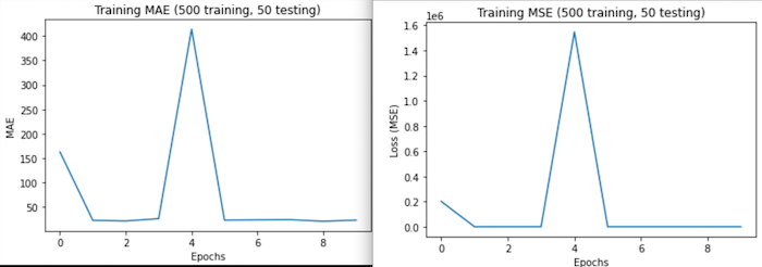
  As evident in the graphs, MAE and MSE are esentially scaled versions of eachother so their graphs will generally have the same shape. In these cases, MSE will have larger values (in the y direction) becuase the distance between the true values and the predicted values was greater than 1 (if the difference (d) is >1, the squared difference d^2>d and if d<1, d^2<d). In these first graphs, there is a sharp increase in error at 4 epochs. This may suggest overfitting after this point, however, I think this is likely because this run used such a small data subset and batch sizes.
  

• Run 2: Next, I increased my batch size to 1,000 training images and 100 test images. I kept epochs, steps_per_epoch, and batch_size the same and had results in under an hour. This time, test loss increased to 877.9531 and MAE to 25.5498. Chalking the decrease in performance up to small batch sizes, I ran the model a third time with larger batch sizes.
  
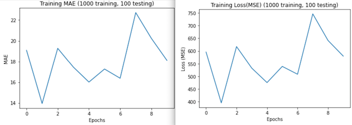
  These graphs show more irregularity than any other graphs. I think this may be a product of providing a large training dataset, while keeping batch size and other paraments small (so the model couldn’t get a cohesive view of the data- its like trying describe what a collection of things look like by seeing a few of them through a straw).
  

• Run 3: For this run, I reused the 1,000 image training set and 100 image testing set and set epochs=10, steps_per_epoch = 10, and batch_size = 100. I kept these numbers relatively low out of fear for miscalculations resulting in insufficient data to complete the fitting process. After 8 hours, the following was returned loss: 878.0463, MAE: 25.5515.
  
  After accounting for an increase in training set size in my model fitting parameters, the results looked more promising. Although my overall test loss and MAE were higher than in previous runs, these graphs show that the model steadily improved throughout training- the lack of irregular behavior in the graphs is a promising sign that the model fit is improving too.
  

• Run 4: Lastly, I increased the number of convolution and pooling layers to 3 each. I fit this model twice- for the first fit, I used a batch size of 10 and for the second, I used a batch size of 50. Other than these changes, I kept my CNN and other fitting parameters the same.
  

Note: After increasing number of epochs for each model, my results changed insignificaly and my accuracy remained at 0.

Run 4(a): Based on my results for run 2, I worried that fitting my model using such small parameters and larger quantities of data would yield poor results, however, the additional convolution and pooling layers seemed to help avoid the irregularity seen in run 2 results. The testing loss (MSE) was just 106.3372 and MAE was 7.5652. Similarly to the graph from run 3, MSE and MAE steadily decreased as training progressed. Additionally, the maximum and minimum values for MSE and MAE were also considerably lower than in the last run.

Run 4(b): This run, I increased batch size to 50. Although it took ~3 hours to complete fitting, I was left with a testing loss of 89.6446 and MAE of 5.9938. Comparatively, these graphs reflect a greater amount of detail (becuase we are working with smaller numbers, visibly smaller change is more significant. An interesting part about this graph is the increase in error at 8 epochs. This increase may be ‘temporary’ and we could see a further decrease in error beyond 10 epochs, however, it may be that the model becomes overfit or innacurate after this point.

Applications: Although my model was highly innacurate, similar models could be useful in the following ways:

• Community growth planning: By imaging large areas and estimating population, community/city growth planners could gauge the number of people impacted by construction, new roads/buildings, natural disasters, and might use this information to determine where expansions could be possible. A modified version of this model might also be able to predict vehicle traffic at certain times/places.
  
• Population growth: Similarly, this model could be used to monitor population growth over time. This technology could also have applications in surviellence and security of high-traffic areas.
  
• Farming and wild animals: On large farms, this model could be modified to track livestock. This model could also be adapted to track specific species in the wild- perhaps a way to monitor endangered species without infringing on their habitat or monitor mass migrations.
  

Ways to improve: My PyCharm will not show matplotlib plots, even with simple examples (it has worked in the past but, for lack of better words, it seems insulted by my numberous long model runs) so I produced the above graphs in Google Colab. This definitely limited what plots I was able to make. If I was able, I would have produced plots of validation MSE, MAE, and accuracy. I would have also produced a plot showing the convolutions for an image, similarly to what we did for the mnsit dataset in the class exercise from the 14th.
In the future, I would like to add more convolution and pooling layers, change the activations, and change the number of neurons per layer, to see how accuracy would change- this would make another interesting graph too (how scores changed over convolutions). Although my model didn’t turn out very well, I learned a lot in the process and would like to try it on images of other areas of the world and different terrains to see how it performs.

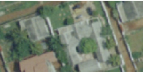
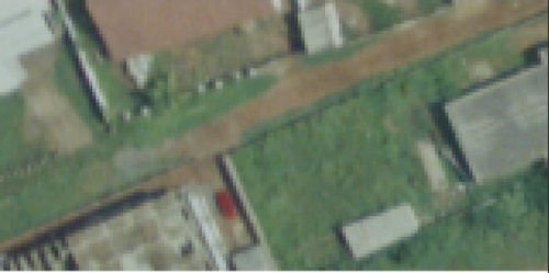
Conclusion: After giving my computer a brief reprieve from fitting, I ran the following images through the model. Unfortunately, the model’s terrible predictive powers shown though.

Model prediction: 20.085924
True value: 36.1680641174316

Model prediction: 18.063229
True value: 24.4707736968994

Model prediction: 18.373161
True value: 35.9370880126953

It is possible that the model is overfit. This is supported by my relatively smooth graphs above and the fact that the model can seemingly only predict values in a small window (~18-20 based on my limited examples above). It may also be that the model is underfit because of the small training set, batch sizes, and low epochs. As I was unable to graph validations error/other scores, I am unable to tell which of these it the case.

Beyond challenges with fitting the model, the data itself also presents some limitations, including:

• From above, a tall appartment building looks the same as a single family home so the model may be incorrectly determining building size incorrectly.
• Non living structures may have been detected and falsely contributed pop size (for example, a livestock barn may appear like a large house from above).