Class exercise (7.14.20)

Question 1: We can use convolutions to improve the performance of neural networks (they reduce the likelihood of over or underfitting). One application of convolutional neural networks is to better train image recognition models. There are several components that allow for the model to work more efficiently, which I will describe next.
Once an image is in black and white, each pixel is assigned a number that idicates the level of color saturation (darker –> higher number). Next, a filter is applied to these pixels. This filter (generally much smaller than the original image) contains a set of values that we can apply to the values of the original pixels. Note that the values of the filter must total to = 0 or 1. If they do not, a weight must be applied that, when multiplied by the total, equals 1. The values of a new, filterd image are determined by scaling each pixel and each of its neighbors by their corresponding weight (entry in the filter) and all these values are then added up. This total is the new value of the current pixel. This process itterates over every pixel in the image, resulting is a transformed image with certain emphasized features depending on the type of filter. This allows the machine to more easily identify sets of features in images that match a label, which improves ‘machine vision’.

Generally: After applying a 3x3 array as a filter (in each case) because the edge pizels of every image do not have neighbors on each size, the dimension of the image is reduced by 2 on each axis.

filter = [ [-1, -2, -1], [0, 0, 0], [1, 2, 1]]
By applying this filter, the resulting image has enhanced vertical lines.

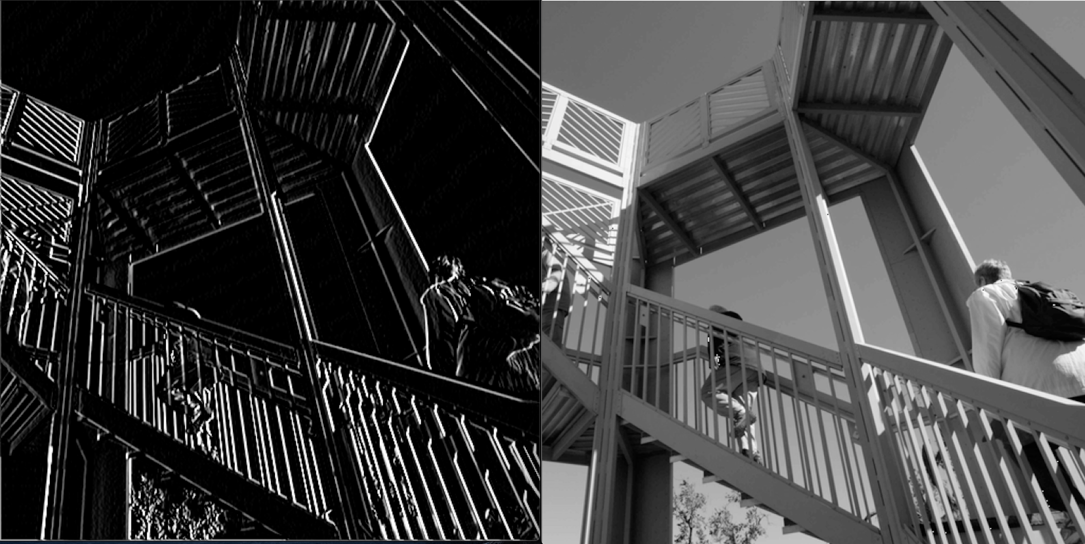
filter = [ [-1, 0, 1], [-2, 0, 2], [-1, 0, 1]]
By applying this filter, the resulting image has enhanced horizontal lines.

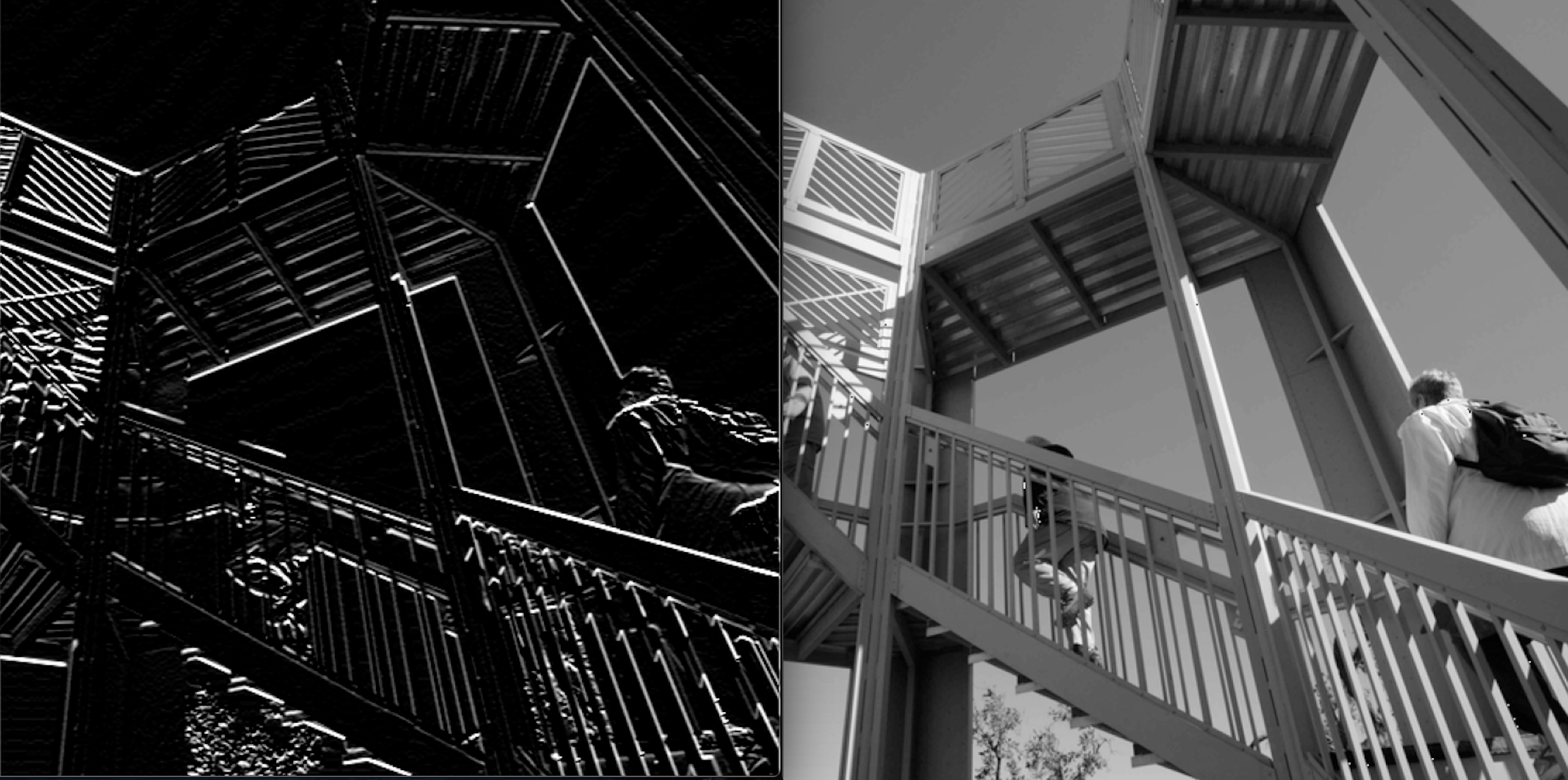
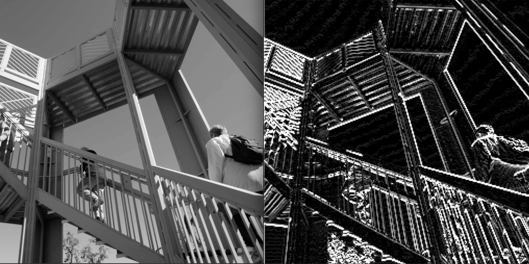
filter = [ [-4, -1, 5], [-2, -2, 4], [1, 1, -2]]

By applying this filter, the resulting image has enhanced areas that were lighter in color in the original image in addition to horizontal lines.

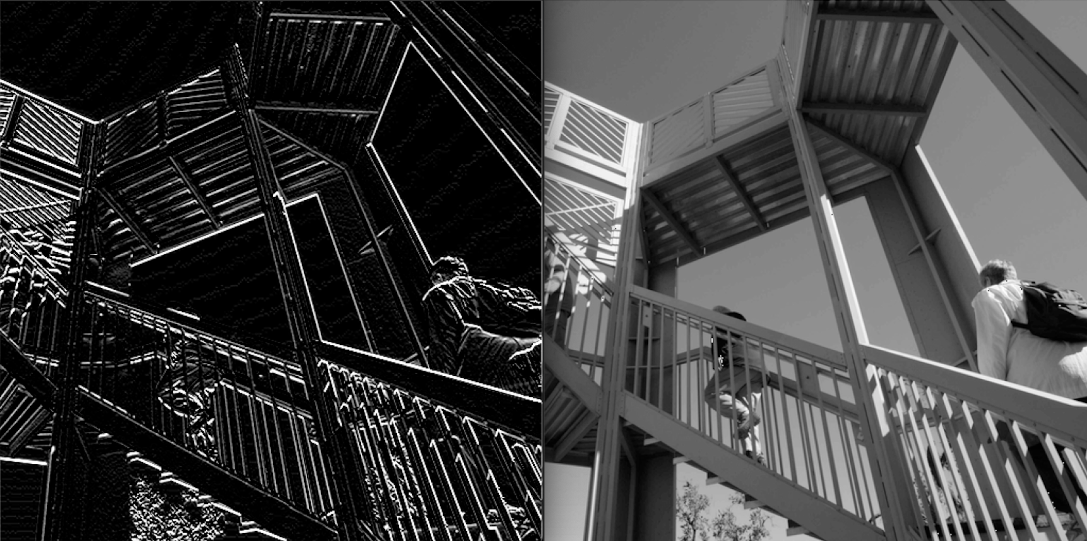
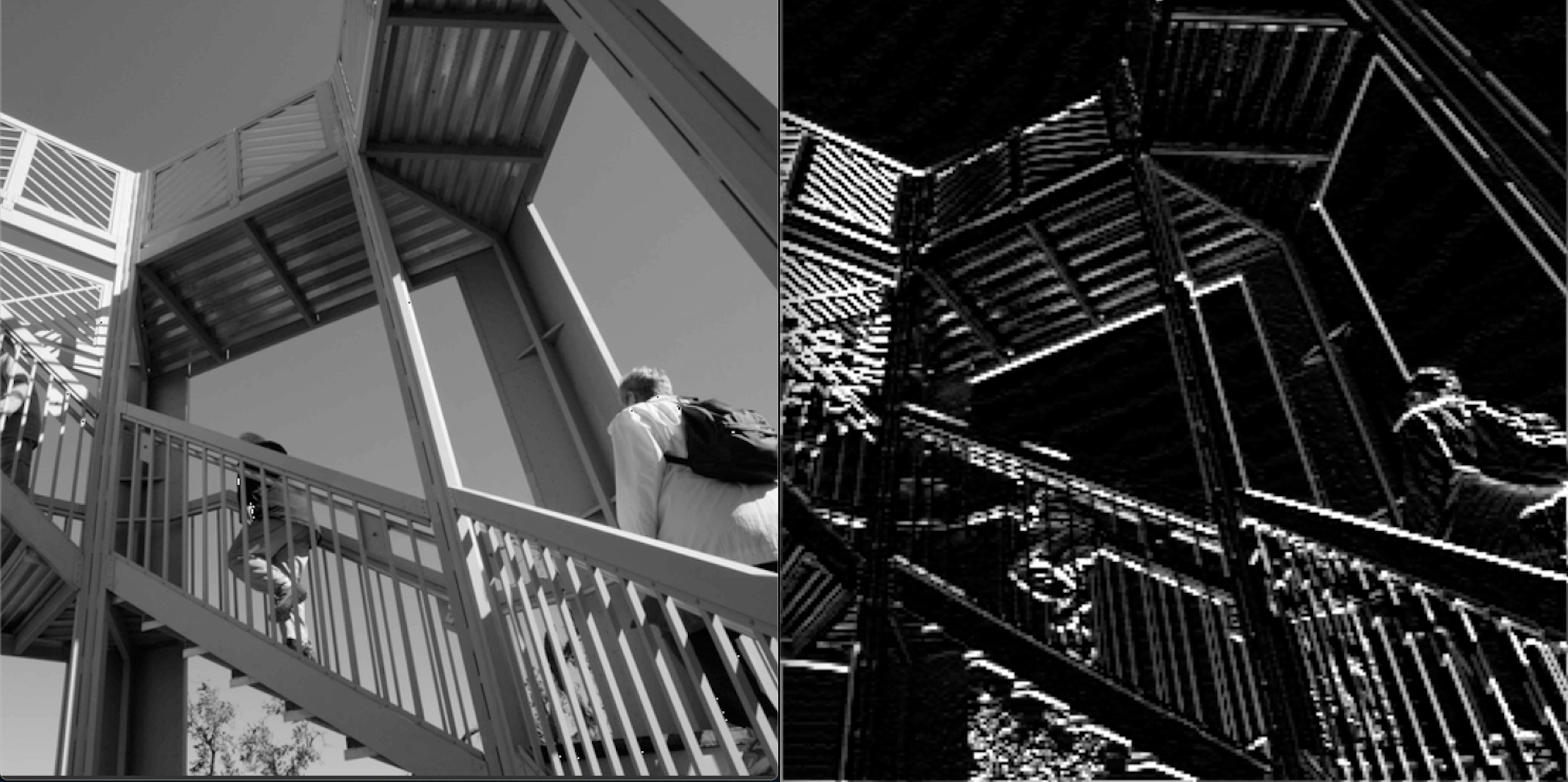
Question 2: The convolutional neural network also utilizes a filter method called pooling. Pooling decreases image resolution, which allows the machine to extract the features it needs while removing extraneous information, making the model training process more efficient while still retaining accuracy. Pooling works by diving the image into a grid with each box containing a specified number of pixels. The function next “looks” at these small boxes and only keeps the largest value. This is repeated for the entire image and the retained values are compiled into a new image containing only the largest values of each subsection (reduces size/resolution). Additionally, because I have my pooling setting to halve the dimension of the image in both directions, the new image is 1/4 of its original size (a 75% reduction in size).

filter = [ [-1, -2, -1], [0, 0, 0], [1, 2, 1]]
By pooling, the resulting image has retained and further enhanced vertical lines with lower image quality.

filter = [ [-1, 0, 1], [-2, 0, 2], [-1, 0, 1]]
By pooling, the resulting image has retained and further enhanced horizontal lines with lower image quality.

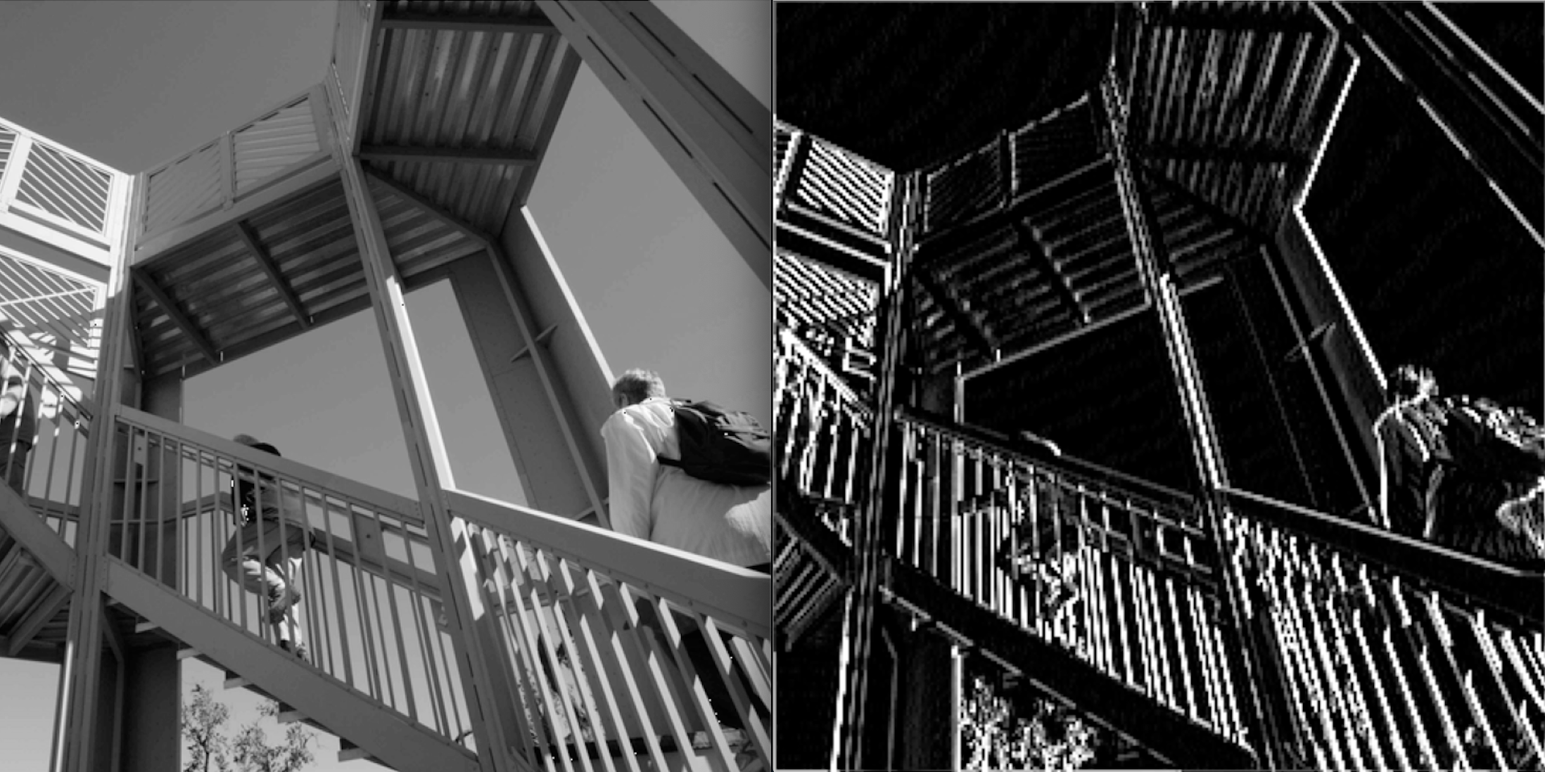
filter = [ [-4, -1, 5], [-2, -2, 4], [1, 1, -2]]

By pooling, the resulting image has retained and further enhanced areas that were lighter in color in the original image in addition to horizontal lines with lower image quality..

Question 3: The convolutional neural network (CNN) greatly outperformed the deep neural network (DNN). This observation is based on the difference in training and testing scores listed below.

DNN: loss: 0.0728 - accuracy: 0.9776
CNN: loss: 0.0258 - accuracy: 0.9925
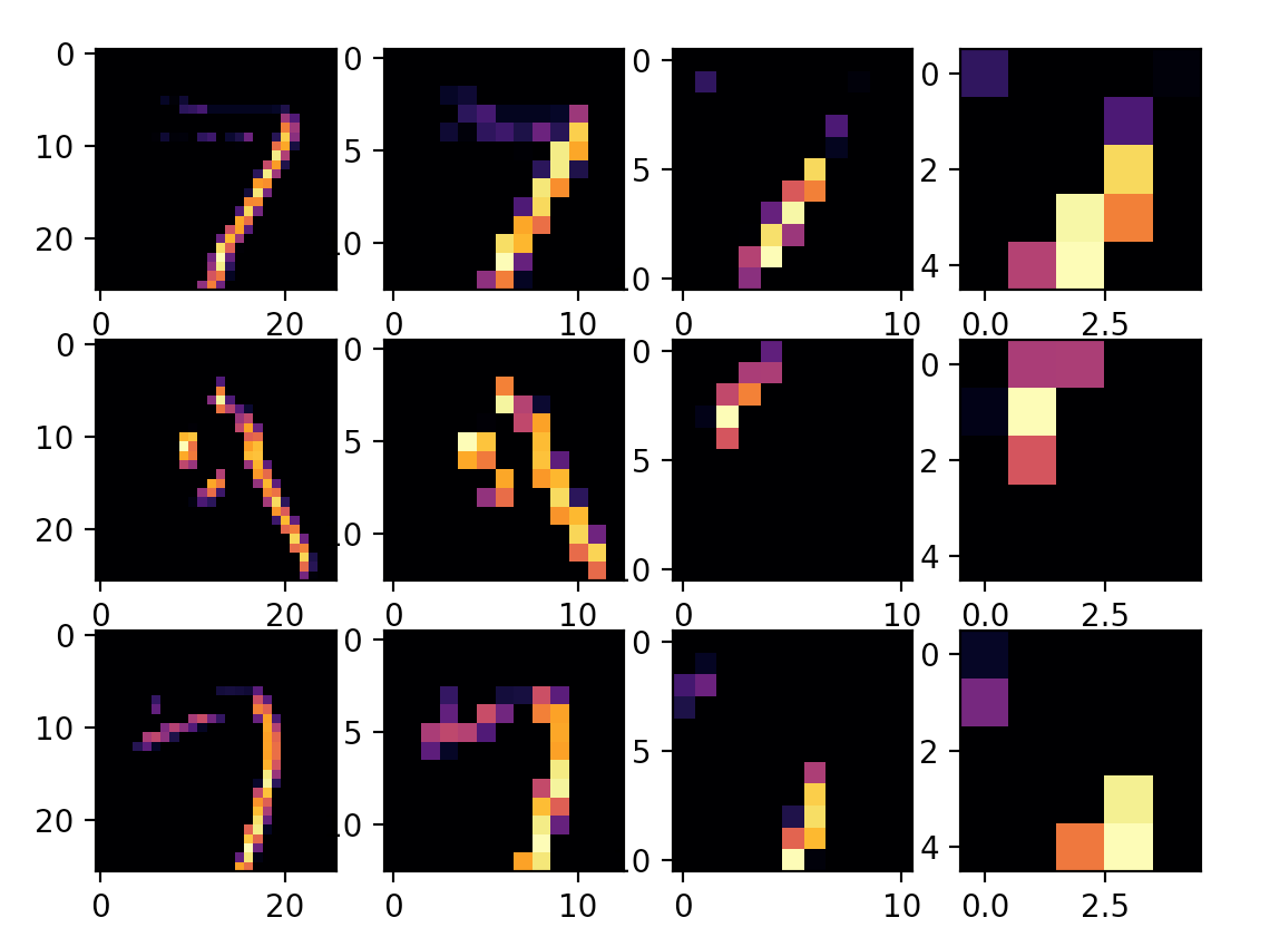
As you can see, using a CNN resulted in lower loss and higher accuracy than the model made using a DNN. It looks like addind the Conv2D and MaxPooling2D layers and waiting out the longer run time for CNN was worth it! Below, the plot shows how the CNN pulls out different features from an image and uses these features to identify the image classification by comparing the features to those is has learned are common to each possible classification.



The number of convolutions is somewhat trivial (it has an affect on model performance but the number has no meaning in the context of the data) and in this case I chose the number 32. If we double this number to 64 (for example), the model’s performance decreases- loss increases and accuracy decreases. This suggests that perhaps the optimal number of convolutions is less than 64 and that additional convolutions may begin to overfit the model.
CNN: loss: 0.0305 - accuracy: 0.9907
Furthermore, if we add more layers of convolutions (from 2 in the previous runs to 3 and using 32 covolutions per layer), we observe yet another decrease in performance! The model is becoming overfit- the loss nearly doubled and the accuracy decreased too.
CNN: loss: 0.0529 - accuracy: 0.9832